Predicting Weighted Sum Scores from plasma biomarkers

library(WSSmod)

Why predict Weighted Sum Scores

Measuring the full proteomic panel is expensive. predict_WSS() instead predicts all 75 module scores of the bundled "core_AD_plasma_biomarkers" reference set from age, sex and eight plasma biomarkers, using a fitted joinet model (a two-layer elastic net) shipped with the package. The vignette Calculating Weighted Sum Scores describes the scores themselves; the modules, biomarkers and prediction model are described in the preprint.

The prediction has two steps:

normalize_wss_biomarkers() puts the raw biomarker values on the rank-based inverse normal transformed (INT) scale the model was trained on.
predict_WSS() returns the module scores.

predict_WSS() needs the suggested packages glmnet and joinet. Chunks below that use them run only if both are installed.

The inputs

The model uses ten columns:

Age, in years,
Gender, numeric, with 1 for male and 0 for not male,
eight raw plasma biomarkers: PlasmaPTau181, PlasmaAB142P, PlasmaAB140P, PlasmaABRatio, PlasmapTau217, PlasmapTau217_AB42Ratio, PlasmaGFAP and PlasmaNfL.

Plasma pTau181, pTau217, Aβ42, Aβ40, NfL and GFAP were measured on the fully automated Lumipulse G 1200 platform (Fujirebio US, Inc, Malvern, PA), following the recommendations of the NACC Working Group. The two ratio columns are derived from these measures (Aβ42/Aβ40 and pTau217/Aβ42).

Example data

The package ships wss_example_biomarkers, simulated values for 20 patients with these columns. They have no biological meaning.

dim(wss_example_biomarkers)
#> [1] 20 10
head(wss_example_biomarkers, 3)
#>           Age Gender PlasmaPTau181 PlasmaAB142P PlasmaAB140P PlasmaABRatio
#> patient01  77      1        1.4203      28.6814     249.8937        0.0963
#> patient02  82      1        2.4113      25.5083     185.1647        0.1052
#> patient03  58      1        2.0431      24.1875     516.0148        0.0783
#>           PlasmapTau217 PlasmapTau217_AB42Ratio PlasmaGFAP PlasmaNfL
#> patient01        0.2373                  0.0053    53.2866   27.6111
#> patient02        0.1343                  0.0017    13.7432   34.9938
#> patient03        0.5072                  0.0175    38.1114   40.8202

Only the biomarkers are normalized. Age stays in raw years and Gender stays 0/1.

# The eight raw biomarker columns, without Age and Gender
biomarker_cols <- setdiff(names(wss_example_biomarkers), c("Age", "Gender"))
raw_biomarkers <- wss_example_biomarkers[, biomarker_cols]

Choosing a normalization

normalize_wss_biomarkers() has two methods. Both return a data frame with the same column names and row names as the input.

`method = "project"` (default)

Each raw value is placed within a bundled reference distribution of baseline values with project_rank_norm(), one biomarker at a time. A value does not depend on the other patients in your data, so this works for a single patient as well as for a cohort.

# One patient
one_patient <- normalize_wss_biomarkers(raw_biomarkers[1, ])
round(one_patient, 2)
#>           PlasmaPTau181 PlasmaAB142P PlasmaAB140P PlasmaABRatio PlasmapTau217
#> patient01         -0.35         0.13        -1.22          0.23          0.53
#>           PlasmapTau217_AB42Ratio PlasmaGFAP PlasmaNfL
#> patient01                    0.04      -0.23      0.75

The same patient gets the same normalized values when scored with others:

# A cohort of 20 patients
projected <- normalize_wss_biomarkers(raw_biomarkers)
all.equal(projected[1, ], one_patient)
#> [1] TRUE

The bundled reference is anonymized: each biomarker’s values were shuffled independently, so it preserves the distribution of each biomarker but not the relationships between them. load_prebuilt_biomarker_reference() returns it.

`method = "self"`

Each biomarker is rank-normalized within your own data with RNOmni::RankNorm(). The result depends on who else is in the data, and it needs at least two patients, so it is appropriate for a sizeable cohort whose distribution you are comfortable normalizing against directly.

self_normalized <- normalize_wss_biomarkers(raw_biomarkers, method = "self")
round(head(self_normalized, 3), 2)
#>           PlasmaPTau181 PlasmaAB142P PlasmaAB140P PlasmaABRatio PlasmapTau217
#> patient01         -0.31         0.19        -1.13         -0.19         -0.19
#> patient02          0.59         0.06        -1.87          0.59         -0.74
#> patient03          0.45        -0.19         1.87         -0.74          1.13
#>           PlasmapTau217_AB42Ratio PlasmaGFAP PlasmaNfL
#> patient01                   -0.31      -0.45      0.45
#> patient02                   -1.40      -1.87      0.59
#> patient03                    0.74      -1.40      0.74

With a single patient it stops with an error:

tryCatch(
  normalize_wss_biomarkers(raw_biomarkers[1, ], method = "self"),
  error = function(e) conditionMessage(e)
)
#> [1] "method = \"self\" requires multiple samples to rank against; use method = \"project\" for a single sample or small cohort."

Which to use

For one patient or a small group, use "project".
For a larger cohort, either works. "project" keeps the values comparable with other data scored the same way and with the model’s training scale. "self" instead centers each biomarker on your own cohort, which suits an analysis of that cohort alone.
Do not mix the two in one analysis.

Predicting module scores

Add Age and Gender back to the normalized biomarkers and call predict_WSS().

newdata <- cbind(
  wss_example_biomarkers[, c("Age", "Gender")],
  projected
)
pred <- predict_WSS(newdata)
names(pred)
#> [1] "base" "meta"

The result is a list of two matrices with one row per patient, named as in newdata, and one column per module:

meta holds the final predictions, from the second layer of the model. These are the scores to use.
base holds the predictions of the first layer alone, before the modules’ correlations are used to refine them. They are returned for comparison.

dim(pred$meta)
#> [1] 20 75
round(pred$meta[1:3, 1:4], 2)
#>           Merged.M17 Merged.M7 Merged.M4 PlasmaPTau181.M26
#> patient01       0.07     -0.16      0.13             -0.22
#> patient02       0.19      0.05     -0.62              0.25
#> patient03      -0.19      0.20      0.45              0.30

The columns are the same modules that calculate_WSS() scores with the default reference set, in the order of the model’s outcomes. A patient scored alone matches the same patient scored in a cohort:

single <- predict_WSS(cbind(wss_example_biomarkers[1, c("Age", "Gender")],
                            one_patient))
all.equal(single$meta[1, ], pred$meta[1, ])
#> [1] TRUE

Reading the scores

A predicted score is on the INT-based scale of the bundled reference set, centered near zero. A higher value means more activity of the module in the direction associated with the core biomarkers, as for measured scores.
Predicted scores are less spread out than measured ones, because a model with few inputs cannot reproduce all of the variation:

# Standard deviation of the predicted scores, first five modules
round(apply(pred$meta, 2, sd)[1:5], 2)
#>        Merged.M17         Merged.M7         Merged.M4 PlasmaPTau181.M26 
#>              0.13              0.28              0.37              0.43 
#>         Merged.M8 
#>              0.20

Compare predicted scores with other predicted scores. They are not directly comparable with scores computed by calculate_WSS() from data on a different scale, such as z-scaled log2 ratios.
Human-readable labels for the modules are in load_prebuilt_terms("core_AD_plasma_biomarkers").

# Spread of the first eight predicted module scores (simulated data, no
# biological meaning), labeled by module term
terms <- load_prebuilt_terms("core_AD_plasma_biomarkers")
labels <- terms$term[match(colnames(pred$meta)[1:8], terms$name)]
par(mar = c(4, 14, 1, 1))
boxplot(pred$meta[, 1:8], names = labels, horizontal = TRUE, las = 1,
        cex.axis = 0.7, xlab = "Predicted WSS score")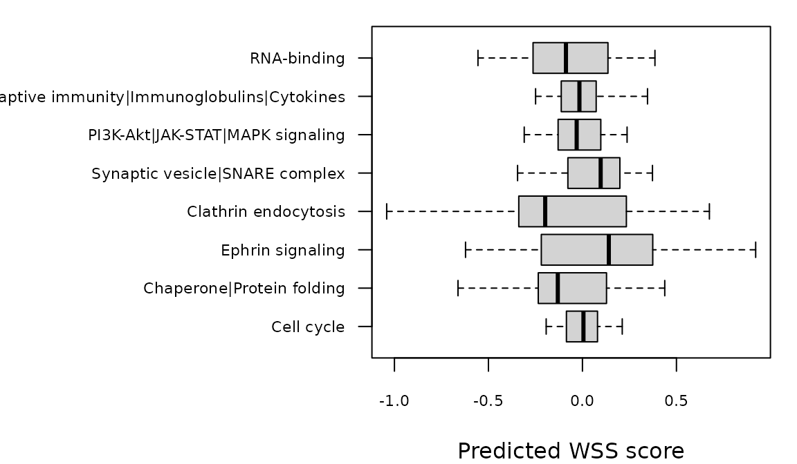

Horizontal boxplots of predicted WSS scores for the first eight modules, labeled by module term, across 20 simulated patients.

Intended use and limits

predict_WSS() is for research use only. It is not a diagnostic tool.
The model was trained on a single baseline cohort. Its performance in other cohorts, assays or populations has not been established.
The biomarker inputs must be measured as in the training data (see “How the biomarkers were measured”). Values from a different assay or platform can produce meaningless predictions even after normalization.
All ten inputs are required, and missing values are not supported.
The data in this vignette are simulated and have no biological meaning.