R6/2 + C31 Biomarkers
- Model: R6/2
- Age: ~4 month
- Drug: C31
- Tissue: Neuroimaging, Urine & Plasma
- Time since last dose: N.A.
- RNA-seq type: N.A.
Table of contents
Publications
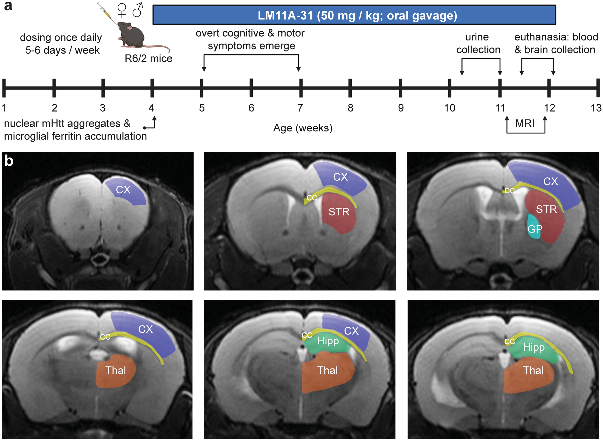
Simmons DA, Mills BD, Butler RR 3rd, Kuan J, McHugh TLM, Akers C, Zhou J, Syriani W, Grouban M, Zeineh M, Longo FM. (2021). Neuroimaging, Urinary, and Plasma Biomarkers of Treatment Response in Huntington’s Disease: Preclinical Evidence with the p75(NTR) Ligand LM11A-31. Neurotherapeutics 18, 1039-1063. DOI: 10.1007/s13311-021-01023-8
Methods
This section is a brief description of the regression and machine learning sections of the paper. The full code is available via the github link above.
For logistic regression, the Z-scaled phenotypes for each comparison were run though sklearn. Snippet below:
def get_log(term, titl):
    '''
    Loops through and graphs log reg importance
    term = list term for _y and _X prefixes, also outname
    saves file returns nothing
    '''
    y = globals()[term + '_y']
    X = globals()[term + '_X']
    model = LogisticRegression()
    model.fit(X, y)
    imp = pd.DataFrame(zip(model.coef_[0],geno_X.columns),columns=['coef', 'feats'])

    fig, ax = plt.subplots(figsize=(16,4))
    sns.barplot(x='feats', y='coef', data=imp)
    plt.xticks(rotation=45)
    ax.set_title('Z-scaled Logistic Coefficients for {}'.format(titl))
    ax.set_xlabel('Feature')
    ax.set_ylabel('Coefficient')
    show_values_on_bars(ax)
    plt.tight_layout()
    plt.savefig('{}.logistic_coef.pdf'.format(term))
    return
For machine learning based feature importance ranking, recursive feature elimination was used to examine all 27 features across a variety of configurations of four two-step ML models (SVM-KNN, SVM-RFC, XGB-KNN, or XGB-RFC). Owing to the small groups, and the goal of robust feature importance assessment. 1000 permutations of the train test split were run for each setup to account for variability in the train test split. Here is an example function for KNN (K_COEFFICIENT=3):
def train_and_predict(train, test, active_features = []):
    knn = KNeighborsClassifier(n_neighbors=K_COEFFICIENT, weights=WEIGHTS_TYPE)
    train_x, train_y = [], train[1]
    for row in train[0]:
        filtered_row = []
        for i in range(len(row)):
            if len(active_features) > i and  active_features[i] == True:
                filtered_row.append(row[i])
        train_x.append(filtered_row)

    knn.fit(train_x, train_y)

    test_x, test_y = [], test[1]
    for row in test[0]:
        filtered_row = []
        for i in range(len(row)):
            if len(active_features) > i and active_features[i]:
                filtered_row.append(row[i])
        test_x.append(filtered_row)

    classes = sorted(set(train_y))
    predictions = []
    for i, row in enumerate(test_x):
        prediction = knn.predict([row])[0]
        predictions.append(prediction)
        probabilities = knn.predict_proba([row])[0]
        prob_str = ""
        for cli, p in enumerate(probabilities):
            if prob_str != "":
                prob_str += ", "
            prob_str += "%d: %.2f%c" % (classes[cli], p * 100.0, '%')

        printer.print ("Prediction for test sample #%d: %.0f, expected %d  (probabilities: %s)" % (i + 1, prediction, test_y[i], prob_str))
    printer.print ("Total prediction score (mean accuracy): %f" % knn.score(test_x, test_y))
    printer.print (classification_report(test_y, predictions))
As noted in the paper, this is a regression use case and not applicable to feature based prediction since the model is most certainly (over)fit to this small experiment. However, the features that scored highly in this analysis would certainly be a good starting point for predictive biomarkers in similar analyses of broader scale.