snRNAseq annotation
Under construction
This page is still being revised. Last update 8/31/2026.
For our single-cell and single-nucleus RNA sequencing projects, we use an iterative clustering process to annotate cell types. This page walks through the current framework, which is built on the Allen Institute whole mouse brain atlas and MapMyCells predictions.
Important
Annotation is a determination, not a lookup. No single tool decides a cluster’s identity — we weigh three lines of evidence together: MapMyCells predictions, marker gene expression, and how the cluster behaves during clustering and QC.
Previous version
The earlier framework (Yao 2021 cortex & hippocampus reference,
class → neighborhood → subclass) is archived at snRNAseq annotation (v1.0).
Table of contents
- The pipeline
- The taxonomy
- Running MapMyCells
- Annotation rounds
- Working through a cluster
- Artifacts
- Marker gene references
- Documentation and review
- Reference files
The pipeline
Annotation sits in the middle of a longer pipeline:
- Raw data processing — Cell Ranger generates counts from the sequencing data.
- Quality control — SoupX removes ambient RNA contamination and DoubletFinder removes heterotypic doublets. Where samples are multiplexed, Souporcell assigns cells to genotypes.
- Integration — samples are aligned with Harmony so that experimental groups can be annotated together rather than separately, and projected to UMAP.
- Automated annotation — MapMyCells assigns each cell a predicted type from the Allen Institute whole mouse brain taxonomy.
- Manual annotation curation — iterative subclustering and review. This is the part you do.
- Downstream analyses — differential expression, pathway enrichment, cell-cell interactions, disease heritability.
Out of scope
Souporcell genotype demultiplexing is only used on multiplexed projects and warrants its own tutorial. It is not covered here.
The taxonomy
Our reference is the Allen Institute whole mouse brain atlas (Yao, 2023), taxonomy version CCN20230722. This replaced the earlier cortex-and-hippocampus-only reference (Yao, 2021), and the hierarchy changed shape in the process:
| v1.0 (Yao 2021) | Current (Yao 2023) |
|---|---|
| Class | (Neurotransmitter type) |
| Neighborhood | Neighborhood |
| Subclass | Class |
| Cluster | Subclass |
| Supertype | |
| Cluster |
Note the shift: what we used to call a class is closer to today’s neighborhood, and today’s class sits where subclass used to. Labels are not interchangeable between the two versions.
A single lineage threaded all the way down looks like this:
| Level | Example | Count |
|---|---|---|
| Neurotransmitter type | Glut | 9 |
| Neighborhood | Pallium-Glut | 7 |
| Class | 01 IT-ET Glut | 34 |
| Subclass | 001 CLA-EPd-CTX Car3 Glut | 339 |
| Supertype | 0001 CLA-EPd-CTX Car3 Glut_1 | ~1200 |
| Cluster | 0001 CLA-EPd-CTX Car3 Glut_1 | ~5300 |
Not every level is hierarchical
Class, subclass, and supertype nest cleanly — a subclass always belongs to exactly one class. Neurotransmitter type and neighborhood do not. A class can span several neurotransmitter types (
12 HY GABAcontains Chol, Dopa, GABA, Glut-GABA and Hist cells), and 29 subclasses are listed under two neighborhoods. Treat those two levels as descriptive, not as parents.
Type is not region is not origin
These three properties are independent, and the labels mix them:
02 NP-CT-L6b Glut(near-projecting / corticothalamic / layer 6b) is consistent across type, region and origin — all cortex/pallium.07 CTX-MGE GABAis a cortical cell that originated in the subpallium, specifically the medial ganglionic eminence, then migrated to the isocortex.
Keeping this straight matters when a prediction looks wrong — see when predictions mislead.
Explore the taxonomy
Hover over a class to see its neighborhood and aggregated marker genes.
Why this stops at class
There are 339 subclasses; they cannot be labelled legibly in a radial layout. For subclass and supertype detail use
ref_tbl(loaded fromoverall.name_schema.csv) and thewmb_dot()marker plots described below.
Running MapMyCells
Draft section
This section documents the mapping step end-to-end for the first time. Verify against your own run before relying on it.
The QC script writes an .h5ad alongside its Seurat output specifically for this step:
R1.<nameset>.postQC.h5ad
Upload that file to MapMyCells and select:
- Reference taxonomy:
10x Whole Mouse Brain (CCN20230722) - Mapping algorithm:
Hierarchical Mapping
Download the resulting zip into your seurat/ directory and extract the CSV from it:
in="R1${nameset}postQC_10xWholeMouseBrain(CCN20230722)"
out="R1.${nameset}.10xWholeMouseBrain"
UTC=$(ls R1*zip | perl -pe 's/^R1.*UTC_(\d+)\.zip/$1/')
7z e "${in}_HierarchicalMapping_UTC_${UTC}.zip" -so "${in}_HierarchicalMapping_UTC_${UTC}.csv" > "${out}.csv"
That CSV is then passed to the clustering script with -m, which joins it into the Seurat object’s metadata. Each cell gains a label and a bootstrapping probability at each level:
| Column | Confidence column |
|---|---|
class_name | class_bootstrapping_probability |
subclass_name | subclass_bootstrapping_probability |
supertype_name | supertype_bootstrapping_probability |
cluster_name | cluster_bootstrapping_probability |
Two sets of predictions
Alongside the MapMyCells columns you will also see predicted.class and predicted.subclass, transferred from a previous in-house experiment (the PS19 + C31 wildtype-vehicle set). We deliberately keep both:
- MapMyCells — hierarchical, so levels cannot contradict each other, and a standardized reference others can compare against.
- In-house predictions — an internal experimental control, and often a better guide to the functional character of non-neuronal cells.
Annotation rounds
Clustering happens at three tiers — overall, then class, then subclass:
| Round | Tier | Notes |
|---|---|---|
| R1 | — | QC, doublet removal, MapMyCells mapping |
| R2 | overall | one clustering of everything |
| R3 | class | one job per class |
| R4 | subclass | one job per subclass |
| R5 | subclass | rerun; repeat as R6 etc. if annotations are still messy |
We never cluster below subclass
Supertype labels are assigned on the subclass-level clusters, not in a clustering round of their own. Typical experiments simply do not have enough cells per type to justify finer granularity. R5 is a rerun of the subclass tier, repeated until the annotations settle — usually four to five rounds in total.
The pipeline scripts live in /labs/flongo/scripts and are on your $PATH on SCG. A single round looks like this:
ml R/4.3.3

# cluster one group at the current tier
02-sc_wkflow_cluster_id.R -n $nameset -r R4 -c "$subclass" -i R4_annots -o R4_annots

# ... annotate in RStudio, export cluster_names.txt ...

# apply the labels and emit the next round
03-sc_wkflow_labels.R -n $nameset -r R4 -T subclass -i R4_annots -o R5_annots
Labels are validated, so copy and paste them
03-sc_wkflow_labels.Rchecks every class and subclass label againstoverall.name_schema.csvand stops on anything it does not recognize. Typos will fail the round. Copy names out ofref_tblrather than typing them.
Breaking these scripts out into a proper documented package is a future goal.
Working through a cluster
Open the annotation notebook for your group, then work through the three lines of evidence for each cluster. Record what you find as you go — the notes are the deliverable as much as the label is.
Clustering and QC behavior
Start by checking whether the cluster looks like a real population at all:
VlnPlot(sc, features = "nFeature_RNA", pt.size = FALSE, group.by = "seurat_clusters")
VlnPlot(sc, features = "nCount_RNA",   pt.size = FALSE, group.by = "seurat_clusters")
VlnPlot(sc, features = "percent.mt",   pt.size = FALSE, group.by = "seurat_clusters")
Our hard cutoffs are 350 < nFeature < 5000 and nCount > 500; typical healthy nuclei land around 2000–4000 features depending on sequencing depth. Very low gene counts with high mitochondrial fraction is a caution flag for an artifact group — with the exception of endothelial and some vascular types, which are legitimately low.
Then check where the cluster sits in the bigger picture. A cluster scattered across the overall UMAP rather than sitting in one place is a chimera candidate:
my_clust <- seq(0, 4)
cell.list <- lapply(my_clust, function(i) {
  rownames(subset(sc@meta.data, seurat_clusters %in% i))
})
setattr(cell.list, 'names', my_clust)
DimPlot(sc1, reduction = "umap.harmony", cells.highlight = cell.list,
        cols.highlight = brewer.pal(9, "Paired"))
Predictions
Look at what MapMyCells called the cells in your cluster, then again with a confidence filter:
table(subset(sc@meta.data, seurat_clusters == 0)$subclass_name)
table(subset(sc@meta.data, seurat_clusters == 0 & subclass_bootstrapping_probability > 0.8)$subclass_name)
Across all clusters at once, a contingency grid is easier to read:
dcast(sc@meta.data, seurat_clusters ~ subclass_name)
and easier still as a heatmap:
a <- melt(dcast(sc@meta.data, seurat_clusters ~ subclass_name))
a$value <- log2(a$value + 0.1)
ggplot(a, aes(x = variable, y = seurat_clusters)) +
  geom_tile(aes(fill = value), color = "white") +
  guides(fill = guide_colorbar("Log2(count + 0.1)")) +
  scale_fill_gradientn(colors = rev(brewer.pal(9, "RdYlBu")), guide = "colorbar") +
  theme(axis.text.x = element_text(angle = 270, hjust = 0, vjust = 0.5))
Predictions spread inconsistently across unrelated types is one of the strongest signals of a chimeric cluster.
Marker genes
The top 30 genes per cluster are generated for you and will separate many of the major types on their own. Beyond those, wmb_dot() plots the atlas’s own markers for a given type:
wmb_dot(sc, type = "001 CLA-EPd-CTX Car3 Glut", tier = "subclass")
It draws up to three panels, and the distinction between them matters:
- overall — general markers of the type.
- tf — transcription factors, which tend to be more robust markers than effector genes.
- within — markers that separate this type from its siblings inside the same parent. Within the
CLA-EPd-CTX Car3 Glutsubclass, its two supertypes are marked byItga8andEgr2— but those genes say nothing useful outside that subclass.
Published reference sets round this out — see marker gene references.
Pathway enrichment
gprofiler2 and Enrichr remain in the annotation template, and you can paste a cluster’s top 30 genes into either. In practice this has not proven very informative off 30 genes alone, particularly now that MapMyCells gives a far more holistic prediction. Treat it as an occasional tiebreaker rather than a routine step.
Artifacts
Not every cluster is a cell type. Bad clusters are labelled, not silently deleted — the four artifact combinations below exist as real rows in overall.name_schema.csv, and labelling them keeps the exclusion auditable:
| Neighborhood | Class | Subclass |
|---|---|---|
| Artifact | Chimeric | Heterotypic doublet |
| Artifact | Chimeric | Low quality |
| Artifact | Dying | Cell death |
| Artifact | Excluded region | (appropriate subclass) |
Dying cells have very few unique genes and often show Ubb, Cmss1, Cst3 and Hspa8 in the top 30, sometimes alongside housekeeping genes like Actb and Gapdh — a sign that nothing cell-type-specific is coming through. They may be disease relevant, but they may equally be preparation artifacts or detritus from lysed cells, so we set them aside and revisit group membership later.
Chimeric clusters carry markers from multiple major groups and get inconsistent predictions. One important caveat before calling a chimera: clustering runs on the top variable genes, so it may fail to split subclasses whose markers did not make that list. A cluster mixing two neighboring subclasses from the same class that otherwise look healthy is probably not a chimera.
Annotations go in the table with your reasoning attached. Real example:
tbl[rank == "subclass", c("7", "10", "11")] <- "Low quality"
tbl[rank == "class",    c("7", "10", "11")] <- "Chimeric"
tbl[rank == "note1",    c("7")] <- "high mito, low nCount & nFeature; predicted for 061 & 062; scattered on overall umap"
tbl[rank == "note2",    c("7")] <- "Slc17a7 & Mobp on Lake & N plot, Mobp on Lake_overall"
tbl[rank == "note3",    c("7")] <- "small cluster in center right mixed with other clusters, near 2, 4, 6, 8"

tbl[rank == "subclass",  c("0","1","2","3","4","5","6","8","9")] <- "062 STR D2 Gaba"
tbl[rank == "class",     c("0","1","2","3","4","5","6","8","9")] <- "09 CNU-LGE GABA"
tbl[rank == "supertype", c("8", "9")] <- "0275 STR D2 Gaba_2"
tbl[rank == "note2",     c("8", "9")] <- "supertype marker Btg2 in top30 (1st for 9)"
Marker gene references
Predictions do not replace marker genes. They remain decisive for two reasons.
Many glial states are not in the atlas. The Allen taxonomy is built for taxonomic classification, but non-neuronal types are frequently studied functionally — they are dynamic, mobile and transcriptionally loud. Microglial and astrocyte supertype labels in particular are often uninformative for our purposes, so we fall back on functional classifications from the literature.
When predictions mislead
Predictions can be confidently wrong when the query lacks context the reference had. A concrete case we hit regularly:
In a whole cortex sample with no striatum present, Lamp5 GABAergic neurons are strongly predicted as striatal GABAergic neurons.
Both populations originate in the caudal ganglionic eminence. Transcriptomic identity appears to track cellular specialization, location and origin together — a compelling hypothesis supported by the Allen Institute’s 2021 and 2023 atlases — so cells sharing an origin can look alike even when one of the two regions was never sampled. The prediction is not noise; it is the reference reaching for the nearest thing it knows. Marker genes tied to cellular identity are how you resolve it.
Plotting reference sets
Two helpers load reference figures side by side with the equivalent plot from your data. Run View(genesets) for the full catalog.
plot_markers(sc, map = "lake_overall")   # violin plots, broad classification
plot_dots(sc, map = "yao_glu_L23456")    # dot plots, finer distinctions
Violin plots give roughly absolute expression and are good for broad calls and for spotting chimeras carrying two sets of major markers. Dot plots give relative expression within groups and are better for fine distinctions and for matching published figures.
Use the tabs below to explore broad marker genes by group.
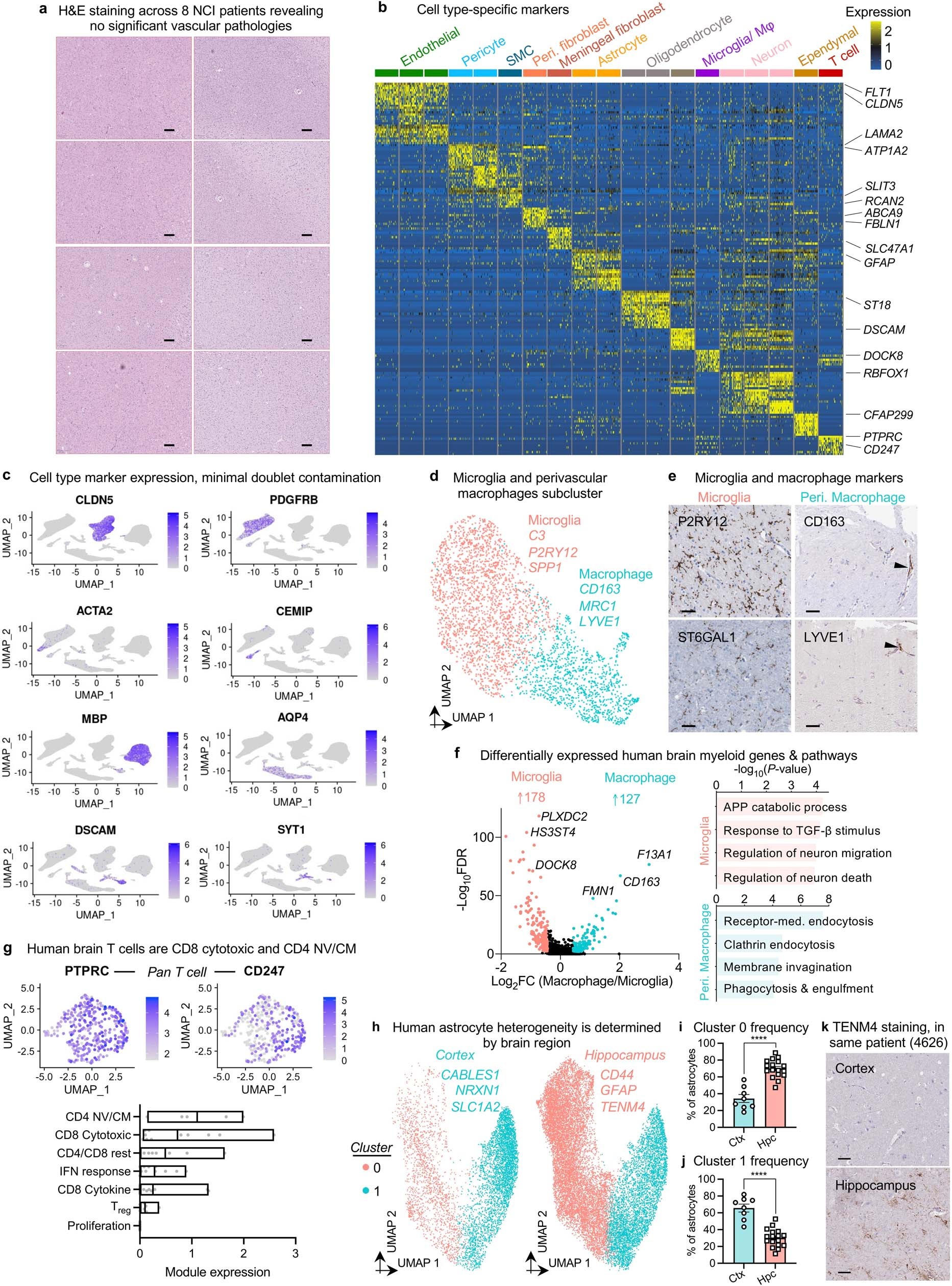
We draw marker genes from the following sources:
- A high-resolution transcriptomic and spatial atlas of cell types in the whole mouse brain (Yao, 2023)
- A taxonomy of transcriptomic cell types across the isocortex and hippocampal formation (Yao, 2021)
- Single-cell transcriptomic profiling of the aging mouse brain (Ximerakis, 2019)
- Integrative single-cell analysis of transcriptional and epigenetic states in the human adult brain (Lake, 2018)
- The TREM2-APOE Pathway Drives the Transcriptional Phenotype of Dysfunctional Microglia in Neurodegenerative Diseases (Krasemann, 2017)
- Human microglial state dynamics in Alzheimer’s disease progression (Sun, 2023)
- Astrocytes and oligodendrocytes undergo subtype-specific transcriptional changes in Alzheimer’s disease (Sadick, 2022)
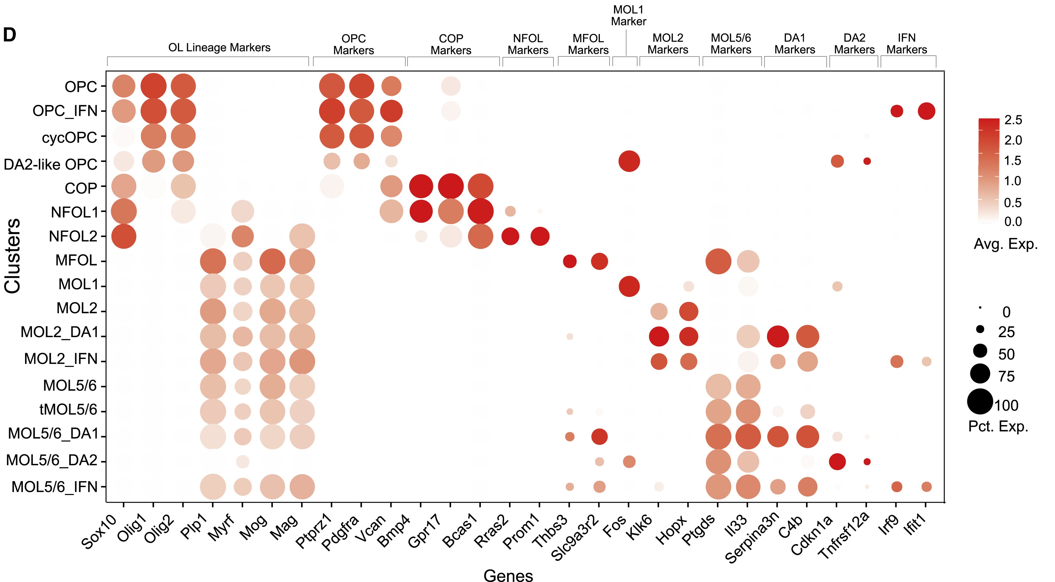
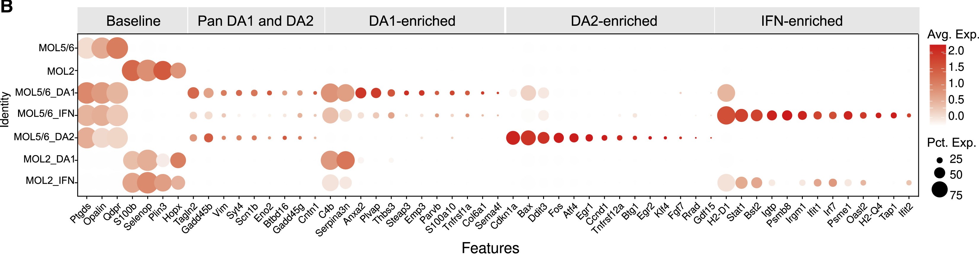
- Disease-associated oligodendrocyte responses across neurodegenerative diseases (Pandey, 2022)
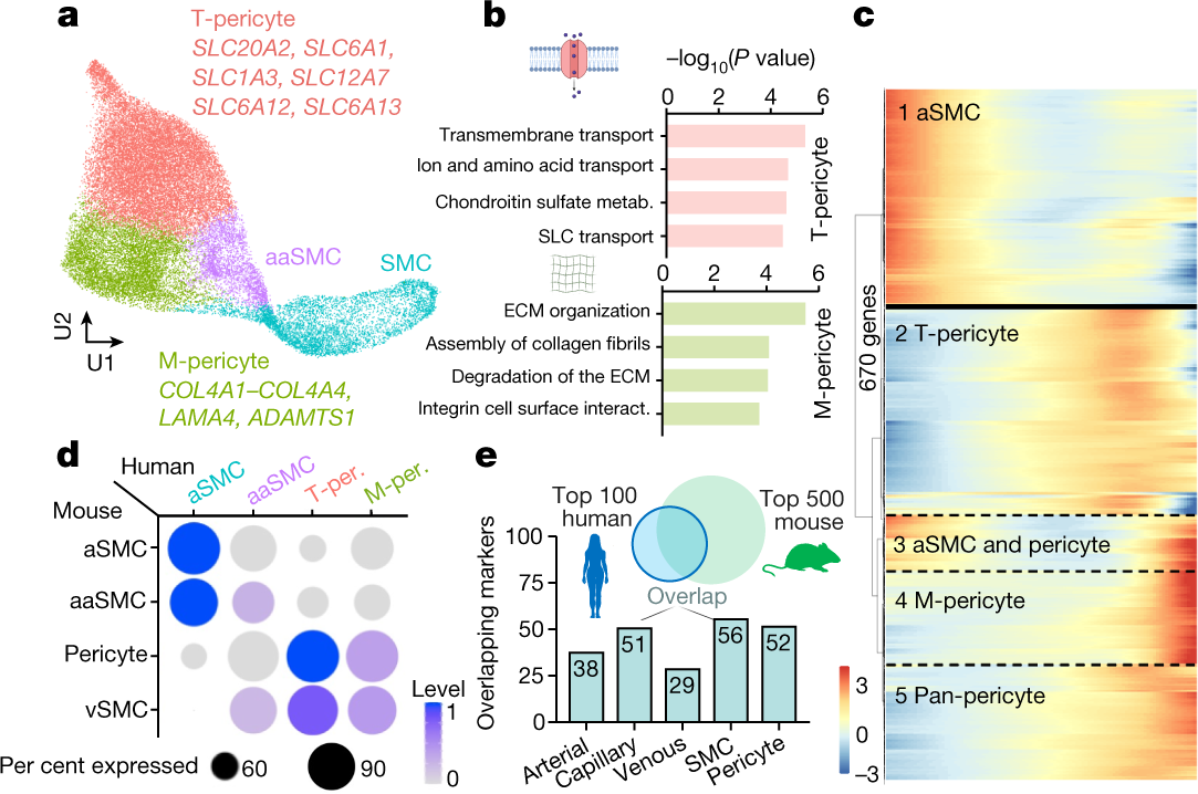
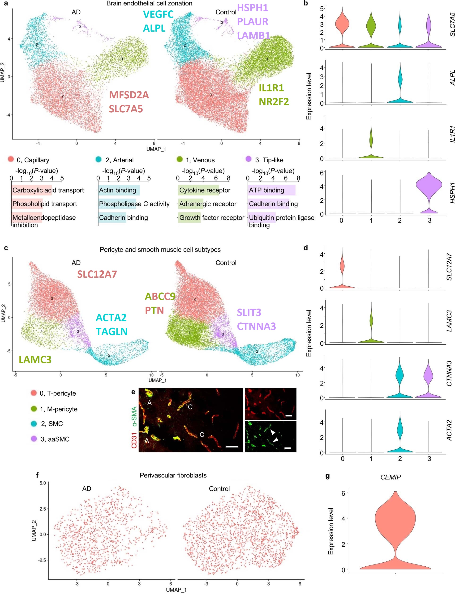
- A human brain vascular atlas reveals diverse mediators of Alzheimer’s risk (Yang, 2022)
Note
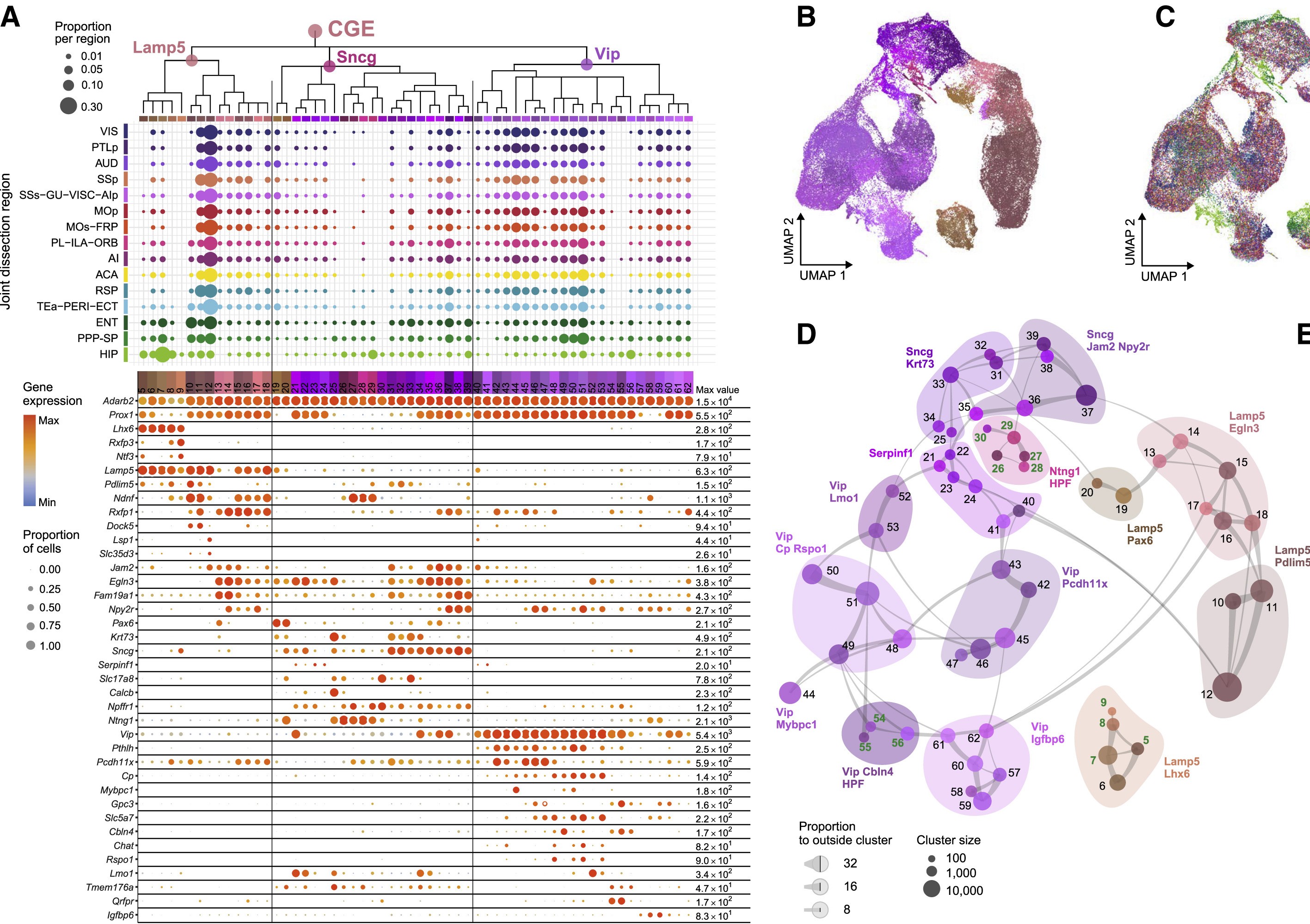
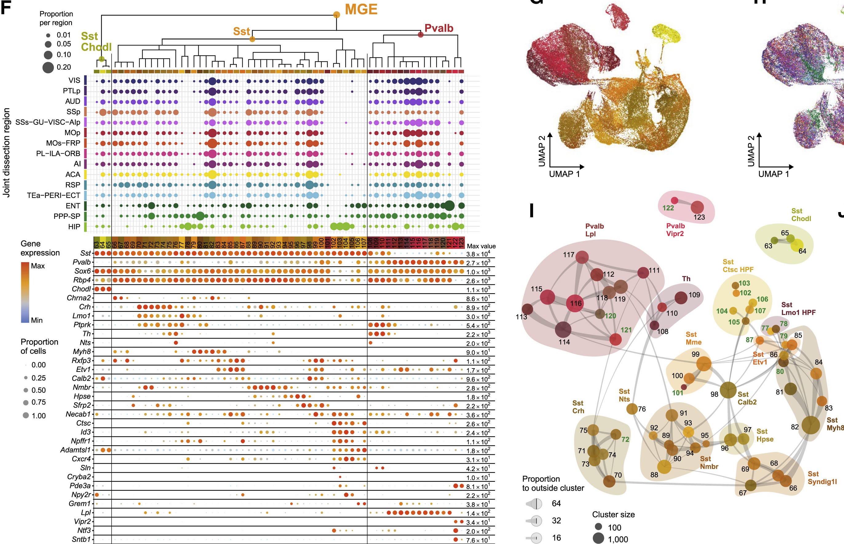
GABAergic neurons of the isocortex fall mainly in the Subpallium-GABA neighborhood, classes 06 CTX-CGE GABA and 07 CTX-MGE GABA.
Caudal ganglionic eminence (CGE)
Medial ganglionic eminence (MGE)
Note
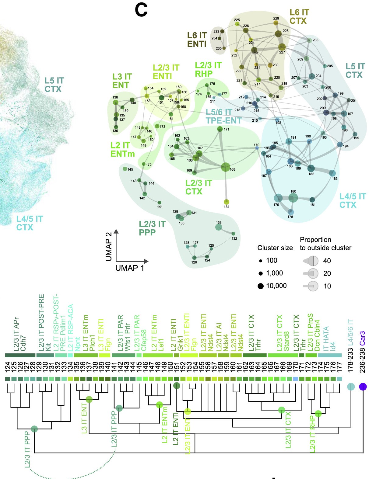
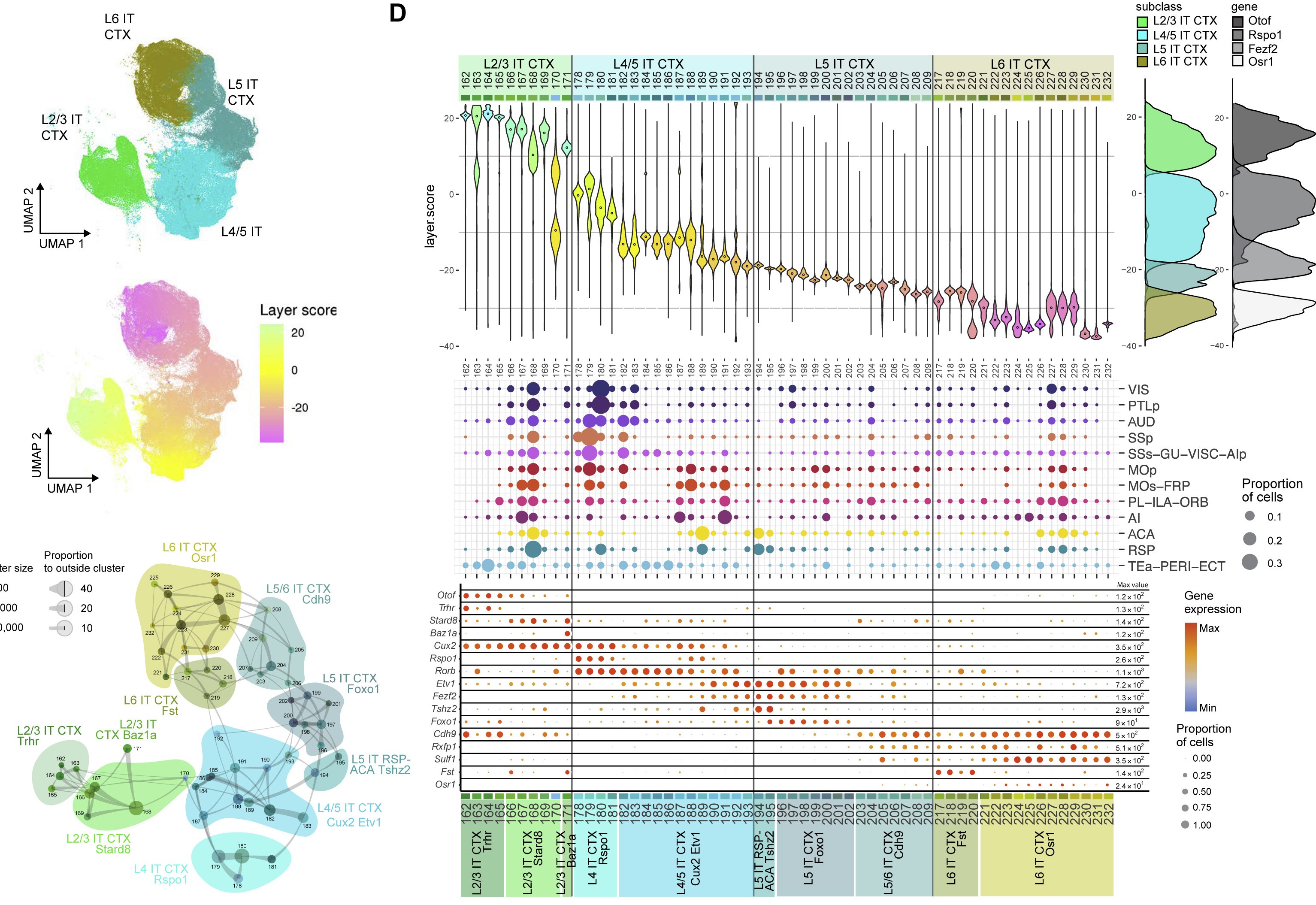
Cortical glutamatergic neurons fall in the Pallium-Glut neighborhood, chiefly classes 01 IT-ET Glut and 02 NP-CT-L6b Glut.
Layer 2/3 intratelencephalic neurons (L2/3 IT)
Layer 4/5/6 intratelencephalic & Car3 neurons (L4/5/6 IT Car3)
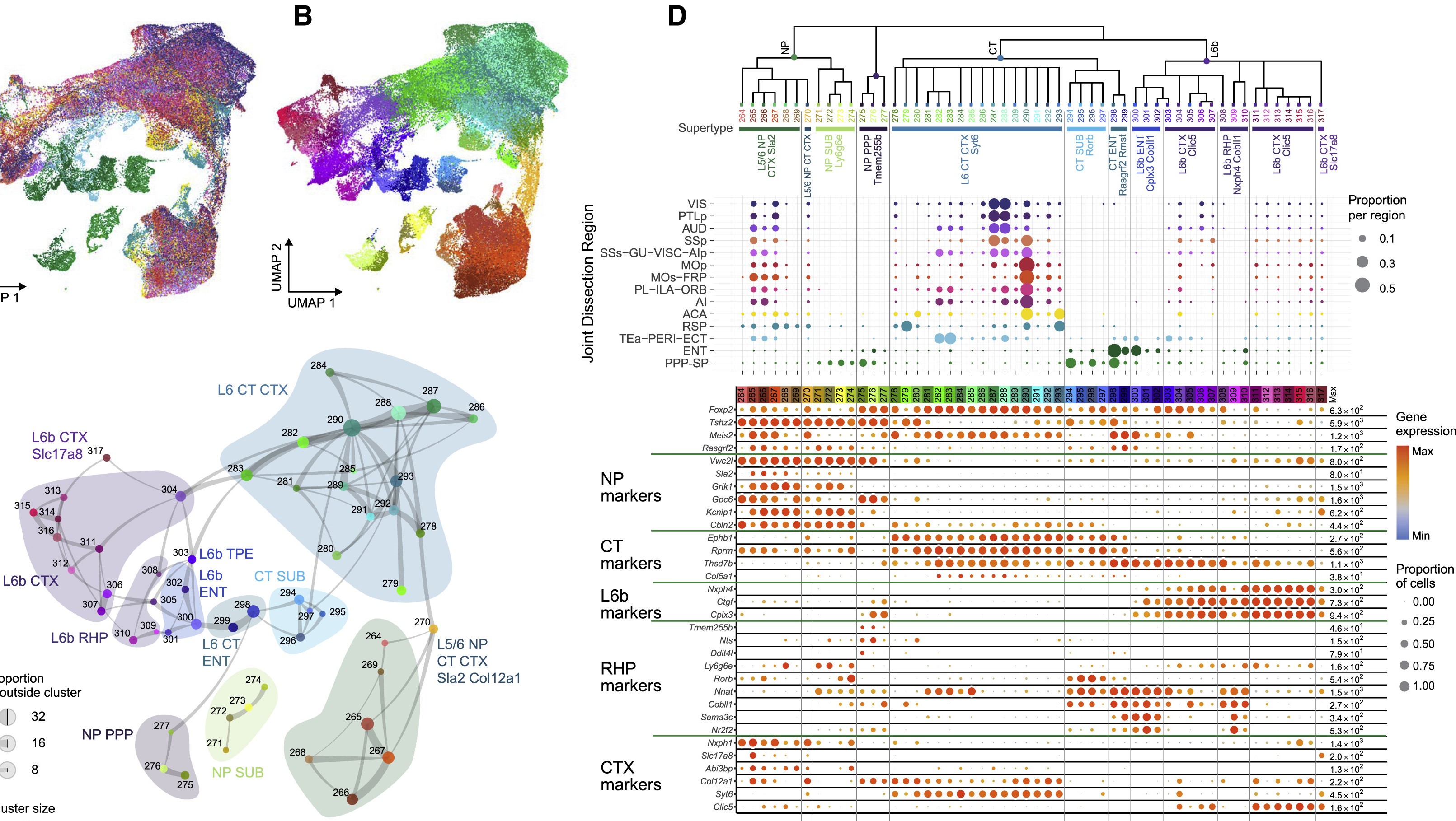
Near-projecting/Corticothalamic/Layer 6b neurons (NP/CT/L6b)
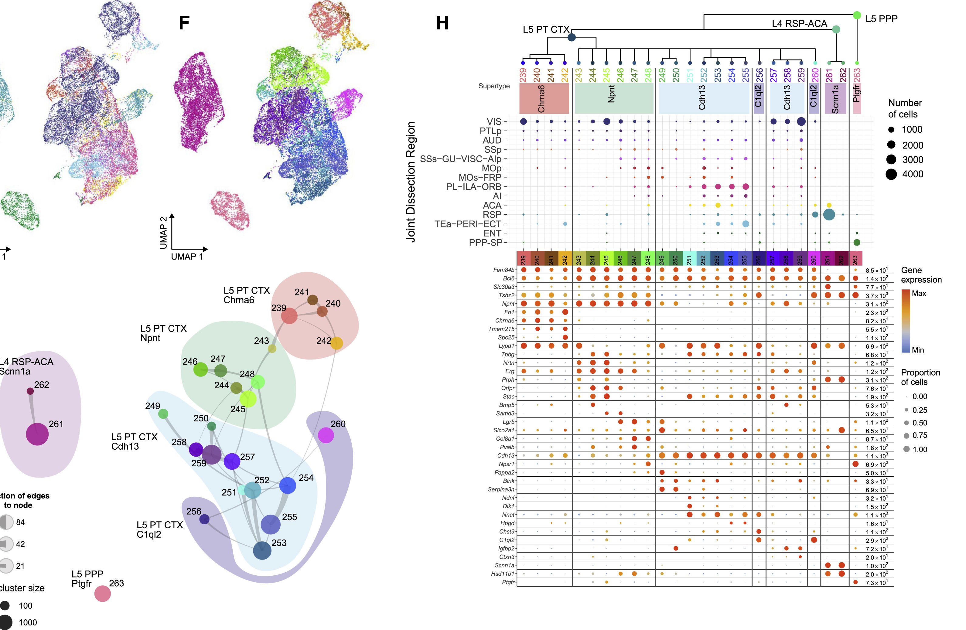
Pyramidal tract neurons (PT)
Note
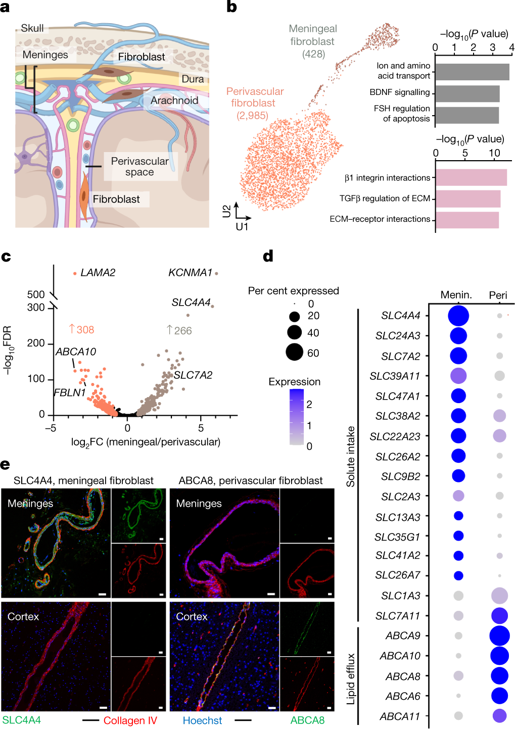
Non-neuronal cells sit in the NN-IMN-GC neighborhood, classes 30 Astro-Epen, 31 OPC-Oligo, 32 OEC, 33 Vascular and 34 Immune. This is where atlas supertypes are least informative and the functional references below matter most.
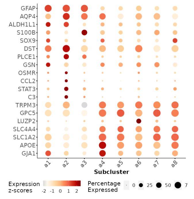
Astrocyte (Astro)
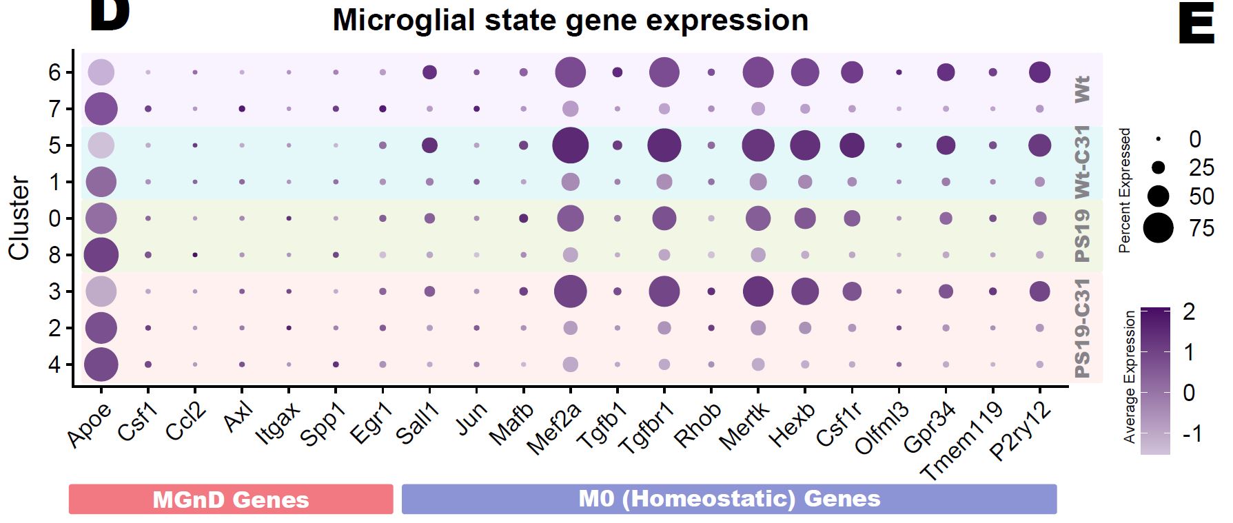
Immune cells (Immun)
Oligodendrocyte precursor cells (OPC)
Vasculature cells (Vascu)
Documentation and review
Every annotation is documented and independently reviewed. This is not bookkeeping — it is what makes the annotations publishable.
- One GitHub issue per annotation. Write your reasoning as you go, and paste screenshots straight from RStudio into the issue. Link related issues with
#. - A second person reviews and you reach consensus. Expect four to five rounds of revision.
- The notes are the point. A reviewer should be able to see how you decided on a type, not just what you decided.
Commit the notebook and annotation table alongside, referencing the issue number:
git add snRNAseq_demo_template_{XX}.Rmd {XX}.top30genes_annot.csv
git commit -m "#1 ready for review"
git push origin main
Reference files
Everything shared lives in /labs/flongo/reference/single-cell:
| File | Purpose |
|---|---|
snRNAseq_annotation_template.Rmd | the annotation notebook, copied fresh each round |
snRNAseq_annotation_functions.R | plot_markers(), plot_dots(), wmb_dot(), get_stacked_bar(), get_genemat() |
snRNAseq_annotation_functions.csv | catalog of available marker genesets (View(genesets)) |
overall.name_schema.csv | the full taxonomy — loaded as ref_tbl, and the source of truth for valid labels |
allen_brain_atlas/ | the atlas workbook and the wmb_dot() marker table |
images/ | reference figures used by plot_markers() and plot_dots() |
To work on SCG, request an RStudio session through OnDemand — 2 cores, 16 GB and 4 hours is a reasonable default, though the overall object needs considerably more memory. Load R with:
ml R/4.3.3
The notebook is interactive
The template uses
runtime: shiny, so it must be run interactively in RStudio. It cannot be knit headlessly.